Chapter 2 Basic R
2.1 Note
This portion of the guide is intended to present you the basics of R to get you up and running.
However, this is not meant to give you all the guidance and know-how, as well as answer all your questions.
There are plenty of internet tutorials already that answer more specific and basic questions.
I’ll provide a few links at the end that complement what I’ll show you here.
2.2 What is R and RStudio
From their own website, simply put “R is a language and environment for statistical computing and graphics.”.
So R is a programming language, just like Python, Matlab or even the syntax you find in SPSS. This language is particularly driven towards mathematical operations and thus proves quite useful when it comes to data management and analysis. Importantly, its an expansive (things keep getting added all the time) and open-source (the code is freely available).
As for RStudio, it is an interface for this programming language. Simply put, it makes working with R easier and everyone (in general) uses this interface to code in R. When you install R it already installs a very basic editor that lets you do some stuff, but RStudio is way more convening for everything other than simple calculations. You can see the basic R editor as Textpad (or Notepad application) and RStudio as Word.
2.3 Why R?
Here follows a list of things R is can do (and excels, pun intended, at):
Read (nearly) all types of data.
Manipulate data in every way possible.
Create any type of graphic data visualization.
Perform any type of statistical analysis.
Perform any type of machine learning applications.
Web scraping.
Creating reports.
Creating web apps.
Many more…
2.4 Where to get it and how to run it
You can download R from https://cran.r-project.org/ and RStudio from https://www.rstudio.com/.
2.5 Environment
This is your basic environment. You have 4 (actually 5 with the upper bar area) divisions.
The top pane (1), gives you access to plenty of options regarding RStudio, letting you open files, save, search, etc..
The pane number 2 is your main area of work. This is your script. The script is the area where you will write your code. This code (all or whatever lines you select) will then be executed in the console.
The console (4) is where your code is executed. You can write single lines directly into it. This is where your information about your errors will show up.
Your right area of the screen contains 2 distinct areas, that can show different things. Area number 3 usually contains your environment. In here you will see every variable that you have attributed (they will be stored here). You can access them by clicking on them. It also contains other sub menus, but I will not go into detail here.
The bottom area (5) contains the files that are in the directory where you area working, will show your plots, will contain your packages (for easy access), the help menu and the viewer (interactive plots pane).
Note, all of your environment is customizable, changing both what panels appear and where, and the overall appearance of Rstudio (you change to dark mode if you think you’re cool enough, for instance).
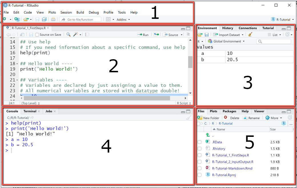
R IDE.
2.6 Scripts, Notebooks and RMarkdown (and Projects)
In creating a new R script you can choose one of three different R documents, R Script, R Notebook and R Markdown.
Well you can actually choose more, but these are perhaps (particularly regarding the focus of this book) the most important ones.
R script is a simple sheet where you write code and add comments by using #. R scripts are best used when are writing scripts for automacy (automating tasks) and don’t necessarily need to view any output along the way, but only at the end (when everything is computed and done). Otherwise, I would almost always recommend either one of the other two formats.
The other two formats are pretty much the same. They only differ in terms of their preview function. These types of special scripts are built with a markdown language, such that the script panel can now be seen as a text document and you can, within that “text document,” insert code chunks and run these code chunk as needed. Importantly, and perhaps one of the best features, is that the output of each chunk is, by default, shown just below that code chunk. This makes these scripts extremely useful when doing data analysis of any kind, given that, provided that they are not too messy, they have the potential to make great reports of your data analysis (showing results and graphs along the way). So if you are new o this, I would recommend using R Notebook otherwise just default to R Markdown.
Lastly, when starting project you can instead opt to first create a Project in RStudio. This will create a .Rproj file in the folder you created your project in. This will help you resume faster your project by simply opening this .RProj and every script associated with the project, as well as the defined working directories will be opened and ready. It has more advantages, such as better integration in version control system such as git, better for collaboration, reproducibility and efficiency.
2.7 Working directories
Whenever you create a new R-type file (e.g., R-script, Rmarkdown, etc.) and you save it somewhere (e.g., “C:/Users/fabio/OneDrive/My Things/Stats/Teaching/R_Book”) it sets your working directory to that folder.
You can change verify this by using the command getwd().
You can also alter this working directory by executing setwd('what working directory I want").
Importantly, when saving your working directory it should in a string format and separated by “/” and not “\”.
For instance setwd("C:/Users/MyName/Work/Project1").
There is also a quick way to do it, although I don’t recommend it as much because the next time you initiate RStudio and work on that script you’ll need to again set the working directory. If you have it in writing in one of the first lines of your scripts it automatically runs it the moment you run your script.
2.8 Operators
R has arithmetic operators and logical operators.
The first ones, arithmetic operators are the following (there are more but, I believe, less important):
+: adds
-: subtracts
*: multiplies
/: divides
^ or **: exponentiates
Then there are logical operators:
<: lesser than
<=: lesser or equal than
>: bigger than
>=: bigger or equal than
==: equals
!=: not equal to
!x: not x
x | y: x OR y
x & y: x AND y
2.9 Classes, Types and Structures
The data you imported can be in a wide range of classes (types). There are 4 basic types of classes, built-in (different functions can use more), you need to be aware (although there are more). These are:
character: Strings (words), such as
"hello"or"hi123".
numeric: Any type of number, such as
2or30.4.
logical: The true or false values.
TRUEorFALSE.date: In a date format. Can be converted from different types (e.g.,
2007-11-11,2jan1960)
You can ask R about what type of object it is by using the class(object) command or the typeof(object)
R also has different data structures. The ones worth talking about here are:
atomic vector: Basically every R data structure. A vector could be a character or an numeric object, for instance.
lists: a list of objects. Can be created by using
list(). You can retrieve the value by using[[]].
l <- list('Potatoes', 4)

l
## [[1]]
## [1] "Potatoes"
##
## [[2]]
## [1] 4my_list <- list('Potatoes', TRUE, 15, c('Strawberry', 1000))
# or
my_list <- list(ingredients = c('Strawberry', 'Milk', 'Coffee'), type = 'Milkshake', rating = 10)- matrix: are like tables.
my_matrix <- matrix(1:9, nrow = 3, ncol = 3)

carro <- matrix(data = 1:9,nrow = 3,ncol = 3)

my_matrix <- matrix(1:9, nrow = 3, dimnames = list(c("X","Y","Z"), c("A","B","C")))- data frame: fancy matrices (more common)
d <- iris
# View(iris)- factor: more of a type of class than anything. This object is a factor with levels.
class(d$Species)## [1] "factor"levels(d$Species)## [1] "setosa" "versicolor" "virginica"- tibble: a special data frame from tidyverse
For additional info, visit: https://swcarpentry.github.io/r-novice-inflammation/13-supp-data-structures/
2.11 Objects
In R you can create objects.
This can be any type of classes we discussed above.
Your object can be a letter, a number, a word, a mix of letters and numbers, a data frame, a vectors, a list, multiple lists, multiple data frames, you name it.
If your object contains multiple things, it becomes a list.
Objects, when created, appear in your Environment panel (top right).
To create an object you must give it a name and then you use <- followed by whatever you want to make an object.
For instance:
a <- 1
b <- 'Hi'
y <- c(1, 'Hi', 3.5)
y <- c(5, 6)
d <- data.frame('Name' = c('Ana','João','Pedro'), 'Age' = c(25, 40, 19))
2.12 Combinations
In R, as you’ve seen above, you can use combinations (concatenations) and attribute these combinations to a variable.
# Create a combination with multiple items.
ctl <- c(1, 'Hi', 3.5)

teste <- c(4, 9, 71)
teste <- teste + 1
teste
## [1] 5 10 72# Asking the mean of that set of items.
mean(x = c(3, 4))## [1] 3.52.13 Subsetting
When you have complex objects (not just a single entry object) you can use subset to select only a specific part of said object.
a <- c('apples','bananas','carrots','oranges','strawberry')

a[1]   # selects first entry
## [1] "apples"a[c(2,3)] # selects entries 2 and 3## [1] "bananas" "carrots"a[3:5] # selects entry 3 to entry 5## [1] "carrots" "oranges" "strawberry"2.14 Ifs and elses
The if() function is a really basic functions in programming languages that allows you to iterate certain actions (i.e., perform an action multiple times).
The if() function is written, and means, the following:
If function
if (condition){
perform_this # if true
} else {
perform_that # if false
}
Here are just a few basic examples for you to get an idea.
# First example
if (3 > 2){
  print('True')
} else {
  print('False')
}
## [1] "True"# Second example
my_list = c('orange', 'banana', 'apple')
if (my_list[2] == 'apple'){
print('The second item in the list is apple!')
} else if (my_list[2] == 'orange'){
print('The second item in the list is orange!')
} else {
print('The second item in the list must be banana!')
}## [1] "The second item in the list must be banana!"2.15 Loops
Loops are also a great tool. These functions automatically run a block of run repeatedly until a end condition is met. You have two types of loops. We will call them the “for” and “while” loops. The latter runs a function, until a “stop” condition is met. I would say while loops are less common, but can be quite useful. However, be warned that they can easily get “stuck”, i.e., you specify a condition that is never met and the loop runs infinitely, forcing you to stop r from running. It follows the following structure.
While loop
while (condition){
perform_this
}
Lets see a basic example of this loop. In this case we have a “my number” object which starts as 0. Then we will have a function that will run until this number is no longer inferior to five. Per each iteration/loop of this function we will add 1 to this number. Let’s see the example below.
# Third example
my_number = 0

while(my_number < 5){
  print('My current number is lower than 5')
  my_number <- my_number + 1
}
## [1] "My current number is lower than 5"
## [1] "My current number is lower than 5"
## [1] "My current number is lower than 5"
## [1] "My current number is lower than 5"
## [1] "My current number is lower than 5"A perhaps more common loop is the “for” type of loop. This type of loop follows this basic structure:
For loop
for (element in set_of_elements){ do_something }
The element can be anything, either a single letter (commonly i, x or z) or a short word. It does not need to have meaning - even though “element” is not known to R, in the context of that loop above it will signify every object in “set_of_elements”.
Ok, so lets work on a very basic example. Let say you have a number “n” and you want to add every number from 1 to 10 to this n. Lets say our initial n is 0 and we want a loop to help us do this without having to do it “manually”.
for (i in c(1,2,3,4,5,6,7,8,9,10)){
  novo_element <- i + 10
  print(novo_element)
}
## [1] 11
## [1] 12
## [1] 13
## [1] 14
## [1] 15
## [1] 16
## [1] 17
## [1] 18
## [1] 19
## [1] 20n <- 0
for (i in 1:10){
cat('\nAdding', i ,'to', n)
n = n + i
cat('\nResult:', n)
}##
## Adding 1 to 0
## Result: 1
## Adding 2 to 1
## Result: 3
## Adding 3 to 3
## Result: 6
## Adding 4 to 6
## Result: 10
## Adding 5 to 10
## Result: 15
## Adding 6 to 15
## Result: 21
## Adding 7 to 21
## Result: 28
## Adding 8 to 28
## Result: 36
## Adding 9 to 36
## Result: 45
## Adding 10 to 45
## Result: 55cat('\nFinal n', n)##
## Final n 55Now onto a more practical one. Lets say you have a list of numbers and you only want to add those that are above 10 to a new list. You could look over every one of them and add it manually, or you could just build the loop below.
my_number_list <- c(7, 20, 21, 5, 61, 2, 29, 02, 19, 44,
                    03, 4, 5.5, 10, 71, 10.5, 4, 65, 4.5)

list_bigger_10 <- c() # empty object

for (n in my_number_list){
  if (n > 10){
    list_bigger_10 <- c(list_bigger_10, n)
  } else {
    cat('\n', n, 'not bigger than 10')
  }
}
##
## 7 not bigger than 10
## 5 not bigger than 10
## 2 not bigger than 10
## 2 not bigger than 10
## 3 not bigger than 10
## 4 not bigger than 10
## 5.5 not bigger than 10
## 10 not bigger than 10
## 4 not bigger than 10
## 4.5 not bigger than 10print(list_bigger_10)## [1] 20.0 21.0 61.0 29.0 19.0 44.0 71.0 10.5 65.02.16 Functions
A function is a set of statements (commands) organized in a way to perform a task.
R, for instance, already has a large number of in-built functions (for instance, mean(c(5, 10, 15)) is a function).
The cool thing, however, is that, as with other programming languages, we can build our own function.
The function takes a set of arguments and performs actions over that argument and output something (if we want).
Its general structure is as follows:
function_name <- function(arg_1, arg_2, ...){
   actions and commands
}
Here are a few examples. Lets say we want to create a function that tells us the square root of our input.
square_function <- function(number_to_be_squared){
  final_number <- (number_to_be_squared)^2
  return(final_number)
}

# Now lets call the function
square_function(number_to_be_squared = 9)
## [1] 81Functions can also be called without arguments.
arg_less <- function(){
  print('Just print this')
}

arg_less()
## [1] "Just print this"They can also have multiple inputs
mult_fun <- function(a, b, c){
  output <- a + b^2 + sqrt(c)
  print(output)
}

mult_fun(a = 1, b = 2, c = 5)
## [1] 7.236068# Or simply
# mult_fun(1, 2, 5)2.17 Packages
There are over 9000 packages. There are packages for nearly everything you want to do. These packages add new functions to R.
You have base packages (already installed, but not loaded) and contributed packages (need to be installed and loaded).
You can install the latter by using the following command install.packages('package_name') and call (load) packages with library(package_name).
Most packages come from CRAN (Comprehensive R Archive Network, which is basically R’s house), thus all you need to write is that.
However, if some packages come from github for instance you need to install the packages “devtools” (install.packages('devtools')) then load it (library(devtools)) and finally use install_github("profile_name/repository") to install the package.
Usually if you google these packages they will have instructions on how to install them.
install.packages("ggplot2")

library(ggplot2)
You can also load and detach (remove package from your toolset for the time being) packages that you have already installed by going to the packages panel (bottom right) and searching and then selecting the package you want to load.
In specific situations, particularly if you just want to use one function of a package, instead of loading the package you can simply write package_name::function_name().
R will just use that function from that package for that line in specific, but not load the package.
2.17.1 Conflicts
Sometimes you will notice that certain packages have the same function names, each with its specific purpose.
There are no conflict on packages loaded by default in R.
These conflicts emerge only when you load new packages (e.g. library("package_name")).
When this happens, R, unless specified, will use the function from the most recently loaded package.
So for instance, in the chapters ahead you will use (and load) a package called “tidyverse”.
When you do call this package (library(tidyverse)) you will already be prompted with a message warning you of possible conflict (although most packages don’t even prompt you with this message).
You can always check what conflicts are currently present by calling the function conflict_scout() from the package (“conflicts”) which is pre-loaded in R.
If you do this further ahead you will be prompted with a similar message:
““” OUTPUT
2 conflicts - filter(): dplyr and stats - lag(): dplyr and stats
““”
Now at least you know that the filter() and lag() functions are shared by two packages.
But remember, each function (depending on the package) has a different… well function.
This might cause you problems when re-running your scripts.
So if you are loading unfamiliar packages or simply have several packages in an R session - a loaded package works for all scripts in a R session, you do not need to load a package for each script! - be wary that conflict might emerge.
Now to resolve this conflict you have three alternatives, which I will present in order of efficiency:
- Use
conflict_prefer("function", "package_prefered")from the “conflicted” package to specify in the R session, which package you always want in regards to that function. So for instance, if I sayconflicted::conflict_prefer("filter", "dplyr"), R will now usefilterfrom “dplyr” in every occasion and thefilterfunction from the package stats will be neglected. - Use
package_name::before each conflicted function to specify which package you want in regards to that function. - Detach (un-load) the package you don’t won’t.
2.18 Shortcuts
Here follows a list of useful shortcuts. Note that these are the ones I can’t live without. There are plenty more, you just have to google them.
- Insert the pipe operator (%>%): Command + Shift + M on a Mac, or Ctrl + Shift + M on Linux and Windows.
- Run the current line of code: Command + Enter on a Mac or Control + Enter on Linux and Windows.
- Run all lines of code: Command + A + Enter on a Mac or Control + A + Enter on Linux and Windows.
- Comment or un-comment lines: Command + Shift + C on a Mac or Control + Shift + C on Linux and Windows.
- Insert a new code chunk: Command + Option + I on a Mac or Control + Alt + I on a Linx and Windows.
2.19 Chunk settings
When using R Notebooks or R Markdown, you’ll work with code chunks, as explained already.
One important thing to know is that these chunks are adjustable, and these adjustments are both easy to make and can come in handy when compiling your code.
These adjustments are made on the top part of the chunk that is between {}.
So for instance, in a normal chunk you have the top portion as “{r}”.
The first parameter tells you which language you are coding in, which in this case is R.
If you are wondering, yes you can change the setting to code in other languages depending if you have them installed and configured with RStudio (e.g., “{python}”).
Besides the language, you can change plenty of parameters.
They have to be separated only by commas.
Below are some brief examples of the ones I most commonly use (all of which, except “fig.width” and “fig.height” are defaulted to TRUE if you don’t set them):
include = FALSE: Runs the code, but does not include the code and the results in the finished file.echo = FALSE: Runs the code, but does not include the code in the finished file (but it includes the results).message = FALSE: Prevents messages generated by the code from appearing.warning = FALSE: Prevents warnings generated by the code from appearing.fig.width = "width_in_pix"andfig.height = "height_in_pix": Set the width and height of the picture/plot.
For more details go to: https://rmarkdown.rstudio.com/lesson-3.html
2.20 Code completion
When you begin to type, R will pop up suggestions as to what you want to write. These can be names of functions, variables or data frames for example. You can press TAB to select and let R auto-fill or just click on it with your mouse.
2.21 Other useful features
Pressing CTRL + F will open up the find/replace menu at the top of your script screen. This can be immensely useful for you to find, and specially, replace lots of things within a portion (the portion you have selected) or the whole code (if you have no code selected).
2.22 Getting help
To get help you have several options, which depend a lot on which type of help you need.
If you want to know what arguments a functions requires, you can write its name and, and having your writing bar inside the “()” press TAB.
If you need generic help about a function - what arguments go where, or, for instance, what does “na.rm” mean in that function - you can use the command ?function_name() in which “function_name” is the name of your function.
This will pop up a help menu regarding that function that will appear on your help panel (bottom right).
You can also click “F1” while your cursor is over the function name.
Depending on the function and its respective documentation this help can either be good or poor.
If you need further help, or need help in problems that are not just concerned about a single function, you will want an internet connection.
Having google searching skills will help lots with your R programming.
A few notes and advices:
- Search your problem using English language.
Search your problem in a generic way using proper searching language (don’t write sentences, write the most relevant words of the problem).
If its an error just post the error message on google.
Don’t be afraid or let down if you need to use google to help you with stuff you learned but just don’t remember. Its normal, trust me.
2.23 Using AI to help you
As of its recent “debut”, another important tool you should consider is ChatGPT by OpenAI. If you haven’t already come across it (launched November 2022), ChatGPT is a chatbot language model. Don’t be discouraged by this wording, its, to say the least, google on steroids, and is particularly useful for programming. However, I cannot emphasize how this is underselling it. I truly encourage you to explore it yourself, and use it as a companion when coding in R. But I would advise some caution when using it, since it can give a false sense of confidence (answers are usually correct, by can lead to mistakes). You should always use your good judgment and search for other helpful tips across the internet.
2.24 Further reading
Need a more in-depth fundamentals of R?
See the links below:
https://www.evamariakiss.de/tutorial/r/
https://www.youtube.com/watch?v=_V8eKsto3Ug&ab_channel=freeCodeCamp.org
2.10 Comments
Commenting your code is good practice. You can comment anything, but perhaps its most practical use is to leave instructions as to what the code, or section of code, is doing.
Commenting is also great for when you don’t want a certain part of your code to run.
Below you see a function, kinda of a confusing one, where comments in each line help me (and other readers) understand what the function is doing.